
You’re diving into statistics or data science, and suddenly you’re hit with terms like CDF and PDF. Your brain freezes. Are these secret codes? Math jargon designed to make you feel lost? Nope!
They’re just tools to help you understand probabilities in a super clear way. Whether you’re a student, a data analyst, or just curious about how probability works, understanding the difference between a Cumulative Distribution Function (CDF) and a Probability Density Function (PDF) is like unlocking a superpower for interpreting data.
In this fun, beginner-friendly guide, we’ll break down CDF vs PDF in a way that feels like chatting with a friend. No boring textbook vibes here! We’ll use simple examples, visuals, and even a YouTube video to make things crystal clear.
By the end, you’ll not only know the difference but also feel confident using these concepts in real-world scenarios like data analysis, machine learning, or even gambling odds.
Ready? Let’s dive in!
What Are CDF and PDF? The Basics
Before we compare CDF vs PDF, let’s get the basics down. Both are ways to describe probabilities, but they do it differently. Think of them as two sides of the same coin—each tells you something about how likely things are to happen.
Probability Density Function (PDF): The Snapshot of Probability
A PDF, or Probability Density Function, is like a snapshot of how probabilities are spread out for a continuous random variable. It tells you the likelihood of a variable taking on a specific value. For example, if you’re measuring the height of people, the PDF shows how likely it is for someone to be exactly 5’6” or 6’2”.
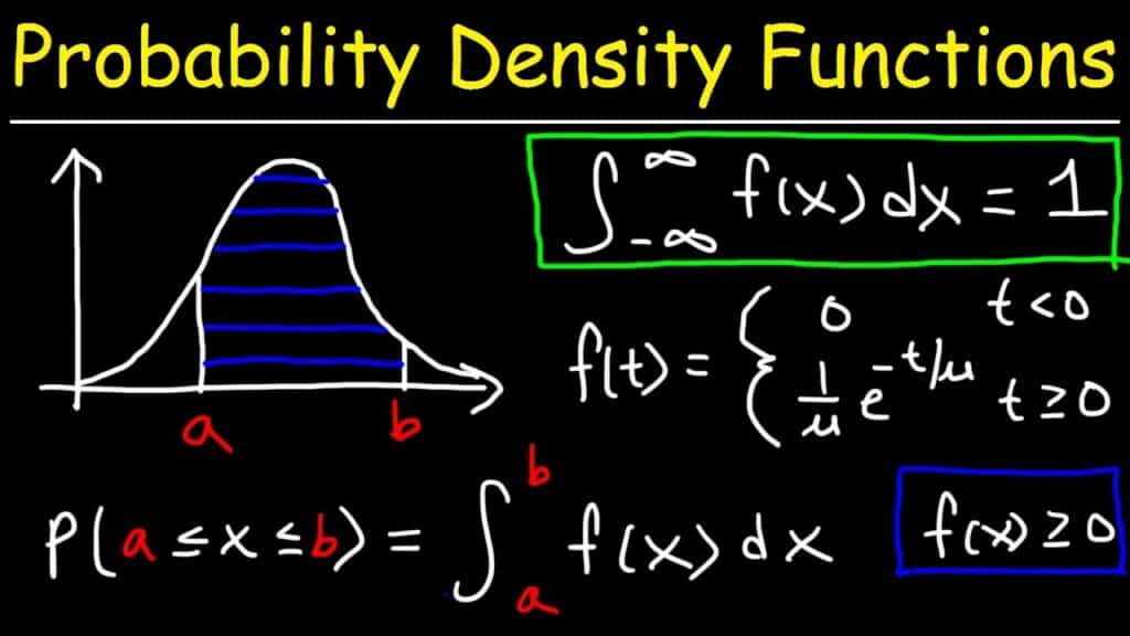
Here’s the catch: for continuous variables, the probability of hitting an exact value (like exactly 5.6 feet) is technically zero because there are infinite possible values. Instead, the PDF gives you a density—a way to measure probability over a tiny range of values.
Example: Imagine you’re rolling a super-fair die with infinite sides (weird, right?). The PDF would show the probability density for each possible outcome. For a normal distribution (that classic bell curve), the PDF looks like this:
Cumulative Distribution Function (CDF): The Running Total
The CDF, or Cumulative Distribution Function, is like the PDF’s big-picture sibling. It tells you the probability that a random variable is less than or equal to a certain value. It’s a running total of probabilities, adding up as you move along the range of possible values.
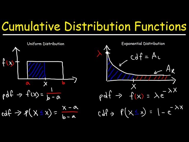
Example: Going back to heights, the CDF would tell you the probability that someone’s height is 5’6” or less. As you move up the scale (5’7”, 5’8”, etc.), the CDF keeps climbing until it hits 1 (100% probability) when you include all possible heights.
Here’s what a CDF looks like for the same normal distribution:
CDF Example
CDF vs PDF: The Key Differences
Now that we’ve got the basics, let’s compare CDF vs PDF head-to-head. Here’s a simple table to break it down:
The Math Behind It (Don’t Worry, It’s Simple!)
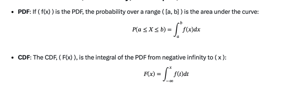
- In plain English: the CDF is the “accumulated” area under the PDF up to a point.
Real-World Example: Imagine you’re predicting rainfall. The PDF tells you how likely it is to get exactly 2 inches of rain. The CDF tells you the chance of getting 2 inches or less. If you’re planning a picnic, the CDF is probably more useful—you want to know the odds of staying dry!
When to Use CDF vs PDF
So, when do you actually use these? Let’s break it down with some practical scenarios:
When to Use a PDF
- Understanding Distribution Shapes: PDFs are great for visualizing how data is spread out. For example, in data science, you might use a PDF to see if your data follows a normal distribution or something spikier.
- Machine Learning: PDFs are used in algorithms like kernel density estimation to model data distributions.
- Example: A company analyzing customer purchase amounts might use a PDF to see the most common spending range.
When to Use a CDF
- Cumulative Probabilities: CDFs are perfect when you need to know the probability of a value falling below a threshold. For instance, what’s the chance a project finishes in 10 days or less?
- Percentiles: Want to know the 90th percentile of test scores? The CDF has your back.
- Example: In finance, a CDF can help calculate the probability that a stock price stays below a certain value.
Pro Tip: If you’re ever stuck choosing between CDF and PDF, ask yourself: “Do I need the probability for a specific value (PDF) or a range up to a value (CDF)?”
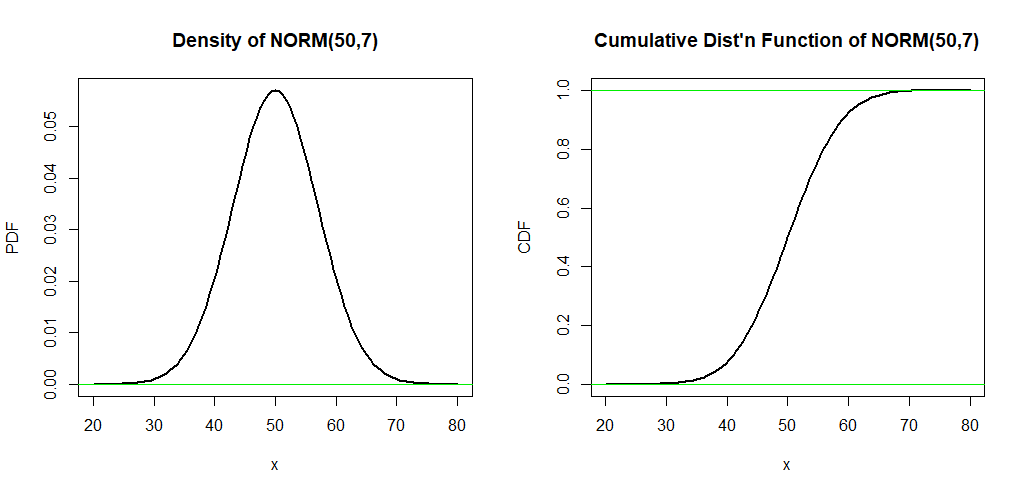
Visualizing CDF vs PDF: A Picture’s Worth a Thousand Words
To really get the difference, let’s look at both functions for a normal distribution side by side:
PDF vs CDF Comparison
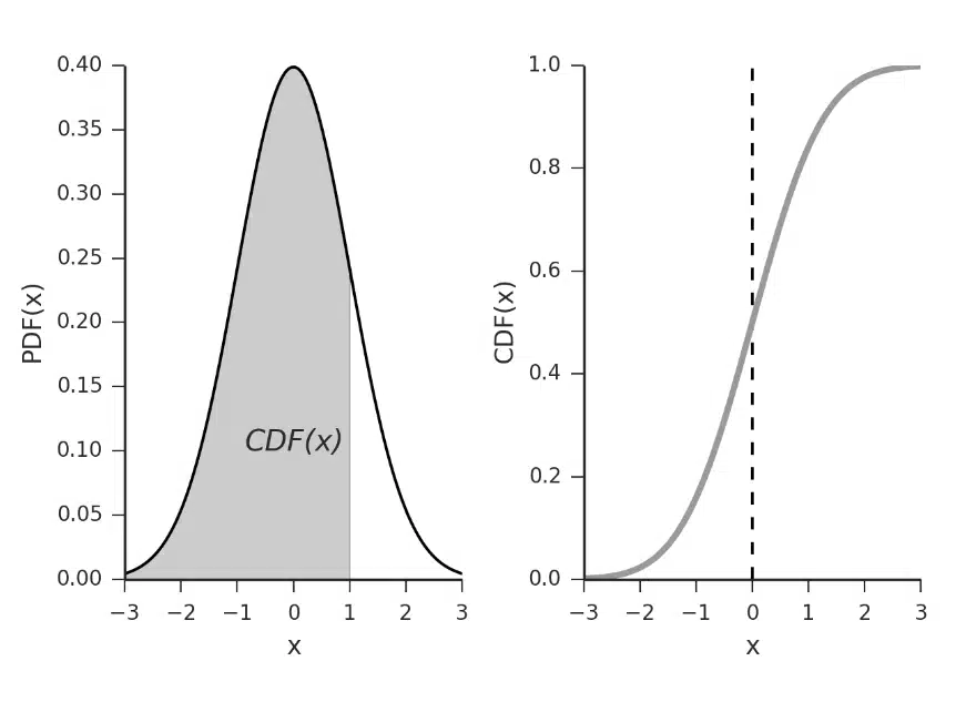
Notice how the PDF gives you the “shape” of the data, while the CDF shows a cumulative buildup? The CDF always starts at 0 (no probability for values below the minimum) and ends at 1 (all possible values included).
For a deeper dive, check out this awesome YouTube video that explains CDF and PDF with animations:
Practical Applications of CDF and PDF
Here’s where things get exciting—how do CDF and PDF show up in real life?
- Data Science & Machine Learning: PDFs help model data distributions, while CDFs are used for tasks like calculating percentiles or evaluating model performance.
- Finance: CDFs are crucial for risk analysis, like determining the probability of a stock price dropping below a threshold.
- Engineering: PDFs model things like signal noise, while CDFs help calculate failure probabilities in reliability testing.
- Weather Forecasting: Meteorologists use CDFs to predict the chance of rainfall below a certain amount.
Example: Suppose you’re a data scientist analyzing customer wait times at a coffee shop. The PDF might show that most customers wait around 5 minutes, with fewer waiting 10+ minutes. The CDF could tell you that 90% of customers wait 7 minutes or less—super useful for optimizing staff schedules!
Tips for Mastering CDF and PDF
Want to nail these concepts? Here are some quick tips:
- Practice with Visuals: Graph PDFs and CDFs for simple distributions (like normal or exponential) to see how they relate.
- Use Software: Tools like Python (scipy.stats), R, or Excel can plot PDFs and CDFs for you. Try coding a normal distribution to see it in action!
- Think Intuitively: PDFs are about density, CDFs are about accumulation. Keep that mental image handy.
- Check Out Resources: Websites like Khan Academy, Coursera, or StatQuest have awesome tutorials on probability functions.
Common Questions About CDF vs PDF
Let’s tackle some FAQs to clear up any lingering confusion:
1. Can a PDF Be Greater Than 1?
Yes! Since a PDF measures density, not probability, its value can exceed 1 over a small range. But the total area under the PDF curve always equals 1.
2. Is a CDF Always Increasing?
Yep! A CDF is non-decreasing because probabilities accumulate as you move up the scale. It never goes down.
3. Can I Convert a PDF to a CDF?
Absolutely! The CDF is the integral of the PDF. Conversely, the PDF is the derivative of the CDF (if it’s differentiable).
4. Do CDF and PDF Apply to Discrete Variables?
Yes, but with a twist. For discrete variables (like rolling a die), you’d use a Probability Mass Function (PMF) instead of a PDF, but the CDF works similarly for both continuous and discrete cases.
Conclusion: You’re Now a CDF vs PDF Pro!
Congrats—you’ve just unlocked the mystery of CDF vs PDF! We’ve covered the basics, compared the two, and explored how they’re used in the real world. Whether you’re crunching data, predicting outcomes, or just curious about probability, you now know that:
- PDFs give you a snapshot of probability density for specific values.
- CDFs show the cumulative probability up to a point.
With these tools in your toolbox, you’re ready to tackle stats problems like a pro. Want to dive deeper? Try plotting your own PDFs and CDFs in Python or check out more probability tutorials online. And if you found this guide helpful, share it with a friend or drop a comment below!